How to Tackle Cavitation in Pump and Propeller Designs with CFD
Pumps | Propeller | Cavitation
Cavitation is a phenomenon in which rapid changes in pressure in a fluid lead to the formation of vapor-filled cavities or bubbles in places where the pressure is relatively low. It can lead to structural damage due to the bubbles imploding when subjected to higher pressure, but it can also cause instabilities and increased noise. Still, it is one of the most challenging topics CFD engineers must tackle. It occurs in many sectors, such as marine propellers, hydrofoils, torpedos, pumps, etc. Many publications cover the subject, sometimes from another point of view, starting from cavitation inception to its actual physical modeling, using pragmatic approaches or more sophisticated models. With this blog article, Cadence would like to share some of its know-how, summarizing state-of-the-art CFD technologies for cavitation prediction and covering different applications and CFD features to answer the engineer’s needs
Cavitation Inception
To study cavitation inception initially, the engineer can be tempted to look only at the pressure level in the 3D field. All places where the scalar field of the total pressure is lower than the vapor pressure are marked so that the total volume of possible cavitation occurrences can be computed. This approach can not give an exact prediction of cavitation and its consequences, but it can already provide good insight. It is what Sirehna from Naval Group did in their publication at Nutts in 2016. Whatever approach is chosen, an accurate pressure field is necessary. Hence, they have used a dynamically and locally refined grid approach where pressure hessian is the most important.
Cavitation Modeling
To model the physics of cavitation, the first method makes use of a single fluid approach. The evolution of density and static pressure are linked through a robust barotropic law, enabling the macro simulation of the cavitation phenomena1. User inputs are minimal, and no additional transport equations are required. The barotropic law is used to evaluate the local density as a function of local static pressure in the cell (Figure 2). According to the local value of density and corresponding vapor pressure, the computational cell can be considered as filled fully with liquid ( = L), vapor ( = V), or a mixture of both. A basic cosinus function determines the profile of the barotropic law in the mixture region.
The barotropic law approach can be easily understood in the example in Figure 3, showing the direct relation between density and local pressure. Indeed, one can see, as the pressure is lower than the saturation pressure, how local density drops to a mixture of vapor and liquid in case the barotropic law is used.
Another way to model cavitation in CFD is by solving an additional transport equation for the vapor mass or volume fraction. Different models like Singhal3, Zwart4, Tani5, Merkle6, Kunz7, Sauer8, etc. exist. The models put the pressure in relation to the saturation pressure to determine a source term based on the Rayleigh-Plesset equation for bubble dynamics. Of course, they require careful treatment and validation of their coefficients. Thermal effects can be included.
When a very precise description of the density in function of pressure and enthalpy is required, the use of thermodynamic tables is suggested. Thermodynamic tables contain the real thermodynamic properties of a particular fluid. They are introduced in the Navier-Stokes equations for mixtures and provide the modeling of the real fluid, taking into account the correct thermo-sensitivity of the saturation pressure.
External Aerodynamic Application
A simple application of the barotropic law is the cavitating flow over a 45-degree conical body (Figure 4), as studied by Rouse and McNown in 1948. The increasing cavitation, determined by the lower cavitation number, is reflected in the streamwise distribution of the pressure coefficient distribution. The barotropic law provides an accurate prediction of the cavitating flow solution.
Turbomachinery Application
A typical cavitation application is the generation of NPSH-Head curves for pumps (Figure 5). This curve shows how the head of the pump will decrease in function of the net positive suction head (NPSH) (the difference between inlet pressure and vapor pressure in the pump). Analyzing the curve on the right, the pump user is informed about the inception of cavitation and till which NPSH they can operate the pump at a specific operating point before cavitation becomes too intensive (usually referred to as NPSHr, for example, corresponding to a head drop of 3%). High cavitation is noticeable as a substantial loss in the head generated by the pump. With the NPSH, a function of the used system, and NPSHr, a property of the installed pump, it’s vital to have this NPSH higher than the NPSHr to avoid pump damage and intolerable noise.
The NPSH-head curve can be computed numerically by increasing the vapor pressure step by step for a defined operating point of the pump. The increasing vapor pressure will result in a decreasing NPSH, a growing cavitation area, and a drop in the pump head when cavitation becomes too extensive. An example is given in Figure 6 for the SHF pump. One can see how the cavitation at the leading edge of the pump blades increases, with the NPSH decreasing until it covers a large part of the blade.
Meshing Strategies
All these test cases have something in common: having a dense and uniform mesh is mandatory since we are looking for local flow particularities, pressure gradients, thin layers, or cavitation bubbles. The correct physics is easily lost or not even captured without such a mesh. Besides, most of the time, cavitation is an unsteady phenomenon and, as such, difficult to predict. Where will it be located? How intense will it be? Questions like these are why a dynamic grid adaptation based on a cavitation criterion has been implemented. During the simulation, the solver adapts the mesh and refines, where necessary, to reveal the presence of cavitation on too coarse meshes. The illustration in Figure 1 is proof of this concept.
Conclusions
The take-home message of the article is that choosing the right path according to the objective is essential. Is it enough to be aware of the presence of cavitation? Should performance prediction be taken into account? How accurate should the modeling be? The answers to these questions will lead to different mesh sizes and a number of equations to solve. CPU time will be impacted accordingly. Mesh density and uniformity are essential in all cases and cannot be neglected.
The good news is that Cadence offers a wide range of tools to model cavitation, accompanied by guidelines for many applications.
Products
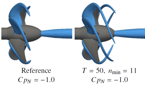 Figure 1: No Local Refinement (left) and Dynamic Mesh Adaption (right)
 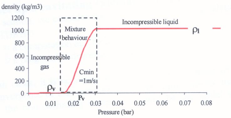 Figure 2: Diagram Barotropic Law
 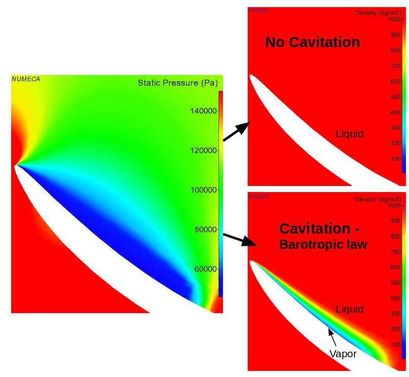 Figure 3: Local Density Drops
 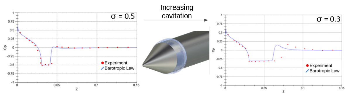 Figure 4: Cavitating Flow over a 45-degree Conical Body
 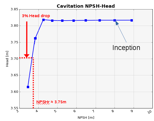 Figure 5: Head of a Pump in Function of the Net Positive Suction Head (NPSH)
 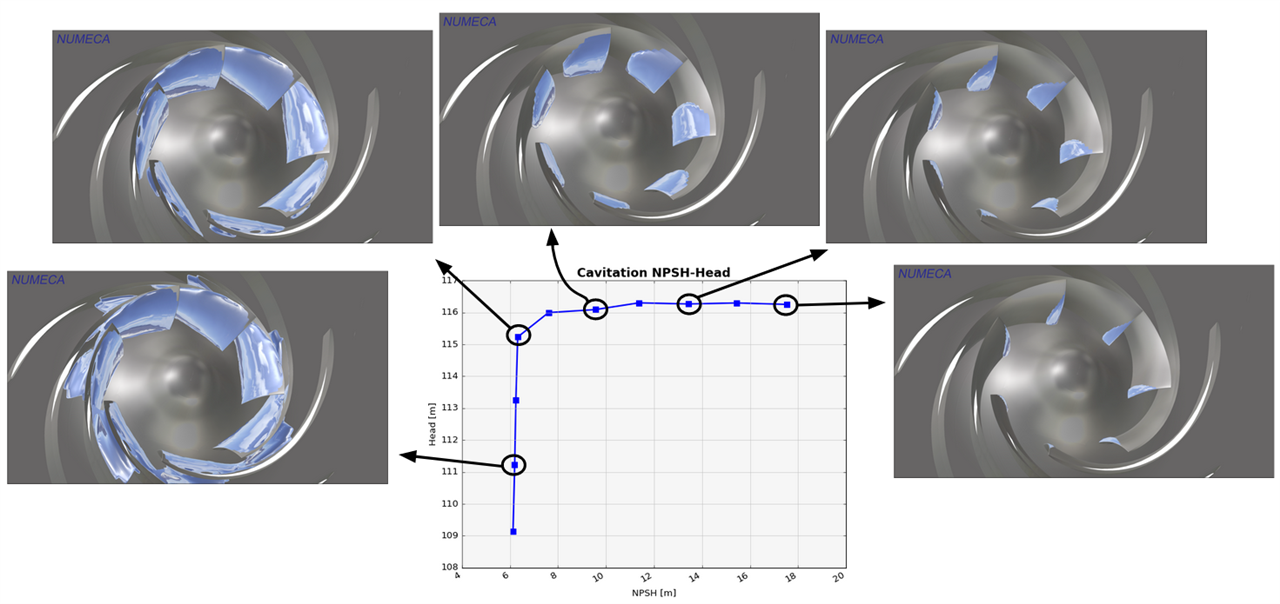 Figure 6: SHF Pump; Cavitation at the Leading Edge for Different Operating Points