An electrified RIVA Powerboat - optimised
Marine | Optimisation | Powerboat
1. Introduction
This work was also presented at the HIPER 2020 Conference in Cortona, and the full paper is available here (page 264).
This paper investigates the hydrodynamic performance of a classic wooden powerboat, the RIVA Junior, using CFD and driven by an environmentally friendly electric motor. The original hull shape is parametrised for variation in an optimisation chain: several operating points (speeds, displacements) and various objectives are considered, aiming to model different operational profiles of an electric propulsion. The goal is to derive hull design trends for both highest speeds for a given power, but also maximised range using the limited electric energy, and of course the trade-offs in between.
2. A short description of the key ingredients
2.1 RIVA Junior and operating conditions
Object of interest is the RIVA Junior hull, a hard-chine motorboat with a single propeller and rudder. With the electric drive and its battery challenge in mind, two displacements are investigated (1m³ and 1.2m³). The idea is to model two powertrain versions (motor, controller, battery) and find the best-possible in terms of speed and range. Furthermore, a large range of speeds is considered, covering the full operating regime:
1) 5m/s: A slow full-displacement mode which might be used near the marina, when aiming for a relaxed ride only, or to save battery to come home safely.
2) 20m/s: A high-speed ride for maximum pleasure and adrenaline.
3) 12.5m/s: A moderate speed mode in between for the rational driver.
- This leads to six operating points per design, which is quite an effort for a high-fidelity CFD simulation with motion coupling and free surface modelling. Some strategies to speed up will be given in the following chapters.
2.2 Parametric modelling and simulation ready CAD
A complex geometry like a planing hull requires a powerful modelling tool, which is CAESES® from FRIENDSHIP SYSTEMS GmbH. A total of 10 free parameters is used, which is a quite low number for the geometric variability it provides. This is a key point, as an increased number of free parameters largely increases the optimisation costs.
2.3 Meshing
The meshing is done in HEXPRESS™, which generates a fully hexahedral unstructured grid with hanging nodes. Some impressions of the mesh are given in Figure 1. The CFD-experienced reader will directly stumble over the missing discretisation along the free surface. For accurate free-surface modelling a fine layer of cells is required perpendicular to the water surface, but in our case these cells will be generated directly in the flow solver using an adaptive grid refinement strategy, see the chapters below.Mesh dependency is investigated using the base design. Since quite a few designs are foreseen in the optimisation, and on 6 operating points, each extra cell will sum up to a quite large difference in total turnaround time. Strongly dependent on the vessel speed and the design this then leads to a final average mesh size of 700k cells.
2.4 Pre-processing and AGR
FINE™/Marine is used as flow solver, a dedicated CFD system for the marine engineer. An adaptive grid refinement technique (AGR) is fully integrated, which adapts (that means refines or de-refines) the mesh during runtime, both in space and time. Several criteria are available, e.g. gradient and overset grid continuity ones, but the widest used are multi-surface ones (free surface or cavitation bubbles, see Figure 2). A dynamic CPU load balancing ensures an efficient CPU usage, so this itself is already a very dynamic system.
2.5 Optimisation strategy
The optimisation toolkit is FINE™/Design3D, which uses Cenaero’s MINAMO package, the optimisation workflow is depicted in Figure 3 and can be separated into three parts:
1) A database containing random samples is generated (the exact method used is called Latinised Centroidal Voronoi Tesselations). The goal is to gain a large diversity and little clustering of design parameters with as little samples as possible.
2) Then an online surrogate-based strategy is used: RANS-CFD simulations are still comparably expensive, which is why the discrete input-output parameters defining a specific design are approximated via a surrogate model to deliver a continuous description. On this the actual optimiser, a genetic algorithm, is applied, calling the surrogate model thousands of times.
3) Interesting candidates are then passed to the CFD chain to get an accurate evaluation of the new designs, and these are then fed back to the database. This is what online stands for in the strategy.
2.6 Efficient CFD chain challenges
The first simulations on even only slightly modified geometries already showed a huge impact on hull resistance and trim angles, but also on the solver runtimes and convergence behaviour. A planing hull is a complex and very dynamic system, and especially the database with random samples can deliver unfavourable geometries. This requires a detailed analysis of such geometries to correctly handle the outputs of interest, find quantities that clearly define such undesired behaviour and, in the end, control the optimisation process and deliver reasonable and consistent data to the optimiser. The latter is of utmost importance, since the surrogate models will of course pick up incorrect data and then mislead the optimiser.
Two extremes are depicted here:
1) Figure 4 shows a random design at 20m/s and fully in the air at the final time step. In this time step the final drag value is of course very low, which is why all the quantities of interest need to be averaged, a window of 30% of the last time steps is used for the final runs. The time-dependant drag also shows a huge oscillation due to the periodic slamming of the hull, and it is visible in the motion variables as well. While the averaged resistance might not be that bad, passenger comfort likely suffers. Hence, calculating the relative standard deviation gives a very good impression of the behaviour and can be used to drive the optimiser. For the optimised samples in this work we use an arbitrary limit of 20% as a constraint.
2) Figure 5 gives an immense bow wave and spray at 5m/s, the total resistance is more than doubled compared to the base geometry. Since the free surface is captured via the AGR algorithm this also leads to largely increased mesh sizes and hence longer simulation times. On the other hand, resistance values will be far more accurate when compared to a static mesh approach, when not using a very conservative (large refinement zone around the free surface) mesh. Hence, over the course of all designs, displacements and speeds the AGR approach surely delivers the most efficient turnaround time.
Another physical property of the hulls is the time to reach a stable hydrodynamic position, if reached at all, and this translates directly into solver convergence and time dependent drag. A convergence checking tool, directly integrated into FINE™/Marine, allows to monitor time histories and stops the process when a given tolerance for e.g. the drag is reached.
Altogether, all those dynamic systems (physics, mesh, convergence) lead to a huge variation in solving time (say 20 minutes to 2 hours per Operating Point on 14 cores), but an efficient trade-off between accuracy and time is found for all those challenges.
3. Results
3.1 Database
The database step is a quite simple one, samples are generated using the defined bounds and the sampling scheme. Depending on maturity of the base design there might already be interesting (equals better) samples in the database, and a key point to check is the accuracy of the surrogate model used later in the optimiser. MINAMO provides this by means of a leave-on-out analysis, which gives the correlation (factor and distribution). Since the genetic algorithm purely relies on the surrogate model, a good correlation is important for a successful optimisation. Also, it can indicate when enough samples are generated to continue to the optimisation step.
A total of 32 samples have been generated in the database, which is on the safe side on most cases in terms of accuracy for ten free parameters. Figure 6 shows the correlation graphs for the averaged total resistance for 5m/s and 1000kg (left) and 20m/s and 1200kg (right). The correlation coefficient for all six drag values are in the range between 0.7 and 0.9, which is very good.
As is expected with the challenges explained above, scattering of the total resistance is quite high. Figure 7 shows the averaged drag at 20m/s over 5m/s, coloured by the value at 12.5m/s. Due to the axis definition all values are negative, and hence the closer to 0 (that is in the top right side) the better the design. The blue cross gives the starting point, that is the Riva Junior base design. Aside from the extreme designs there are already some good designs, which show substantial less drag.
3.2 Optimisation
In this work only one set of multi-objective optimisation run is shown: the Pareto type optimiser uses all six averaged drag values as objectives and the relative standard deviation of the drag is specified as constraint to be less than 20. Of course, there would be room for many more sets of objectives and constraints, but the following results already show quite good results overall. Vessel motion variables are also evaluated, but except from the flying/slamming hull type these values are not excessive and hence not deemed necessary as objectives. Also, the overall physical behaviour of the hull is well represented by just the time evolution of the drag, and its standard deviation.
Figure 8 shows the total resistance values, this time without a colormap for the values 12.5m/s. Blue dots indicate database samples, orange ones are coming from the optimiser, while small dots indicate non-feasibility (here: drag deviation constraint of 20% not met). Again, the results seem very good and indicate a successful optimiser run. There are no samples in the completely un-usable region, showing a very good prediction from the surrogate model – high scattering here would point in that direction. There is also only a small amount of non-feasible designs.
Figure 9 shows again a zoom and giving all resistance values per displacements. In total 56 samples were generated during the optimisation run, which is not that much regarding the complexity of the problem. Still there are already many samples that indicate the Pareto front, and by just judging from the penalties design number 79 (marked with a star) shows a very good overall performance. At a displacement of 1m³, resistance at 5m/s is reduced from 1160N (all values shown in the plots are for half ship models) to around 1000N, which is around 13%. At 12.5m/s, the reduction is from 1760N to 1560N, translating into 11%. The highest speed of 20m/s shows the greatest improvements, total resistance is decreased from 3630N to 2340N, hence 35%. This design can also keep these improvements at 1.2m³ and is hence seen as optimal in respect to all six objectives.
These figures also show another important advantage of the Pareto-type optimisation: there are several other candidates found which are probably not as balanced as design 79, but favour objectives in respect to others: this is the strength of a true multi-objective algorithm with a wide range of very good potential designs. Looking at 1m³: design 48 is slightly worse at 5m/s compared to number 79 and can almost keep the performance at 20m/s, but it shows another 6.5% decrease at 12.5m/s, hence this could be a hull shape for a light battery configuration with great endurance at already planing conditions (water-skiing comes into mind), and still has the potential for thrilling high-speed driving.
A final word on the overall turnaround time: a 28-core machine is used for the database and optimisation, running two operating points in parallel on 14 cores. The database took only a couple of days, and the optimisation was completed in around a week (pure CPU time), which is very fast considering the complexity and the small machine used.
3.3 Data Mining
The procedure shown here produces a lot of data, and so far only new designs and their performance improvements are discussed. But, using this data and applying so called data-mining tools can greatly increase the understanding of physics and the correlation to input parameters. Figure 10 shows one of those tools, the self-organising maps (SOM). They are also based on a surrogate model, and project high-order data (here a problem with ten input parameters and six objectives) into 2D space. Each point indicates a design of the database and optimisation loop, and it is fixed in space. The colour contours display the total resistance values for all three speeds (rows) and the two draughts (columns). Note that red means low resistance and blue a high one. There is a strong correlation between all six performance values on the top left side of the SOMs, and a very favourable area at full displacement speed (5m/s) on the bottom right. The planing modes are strongly focusing on the top right side, especially for 12.5m/s, while at 20m/s the bottom part is also attractive.
These plots clearly show that trade-offs must be made when aiming for a Jack of all trades design, and number 79 (marked by a star) is very good overall. There are samples which favour either of the operating modes, but at the cost of others. Again, the designer or engineer needs to decide what he or she wants.
Another useful tool is the analysis of variance (ANOVA). It is also based on the surrogate model and allows to calculate the sensitivity of all input parameters in respect to the output, here resistance values. Figure 11 gives the ANOVA plots for all six operating conditions in this study. The rocker parameter, which impacts the keel line towards the transom, is quite dominant for all planing conditions (12.5m/s and 20m/s), although a bit dependent on the displacement: it is far more impacting on the light version than on the heavier one. Total boat length on the other hand is a strong factor for the displacement speed, while completely irrelevant for high speeds.
ANOVA can hence guide a designer in a lot of ways: for example, it can show sensitivities which were probably not known before and need to be considered much more in the next project. This can be a change of parametrisation for finer control over important features and paving the way for even better designs. And the opposite might be true as well: less important features can be neglected, which in a workflow similar to the one presented here will save CPU time, or in the real world could also save material or costs in general.
4 Conclusions
An optimisation of a small powerboat has been presented, using numerical simulations. One focus lied on the application of electric propulsion instead of a combustion engine, which brought a few extra challenges with it: battery size is a crucial parameter and was respected using two different displacements. The full operating range, from low to high speeds was considered, to allow for a complete picture of such a powerboat. A powerful combination of efficient parametric modelling using CAESES® and state-of-the-art CFD solutions from NUMECA led to a very stable, yet cost-effective design process. The results of the optimisation run were quite promising, showing some major gains in terms of total boat resistance. A few designs were discussed in more detail, showing some trade-offs between the six operating conditions. A deeper look into the results and the vast amount of data was given via data-mining tools, that can easily show trends, correlations and anti-correlations in the design space. Also, sensitivity analysis methods were applied to highlight a few of the important geometrical features of such a boat.
Author
Sven Albert, NUMECA Ingenieurbüro
Products
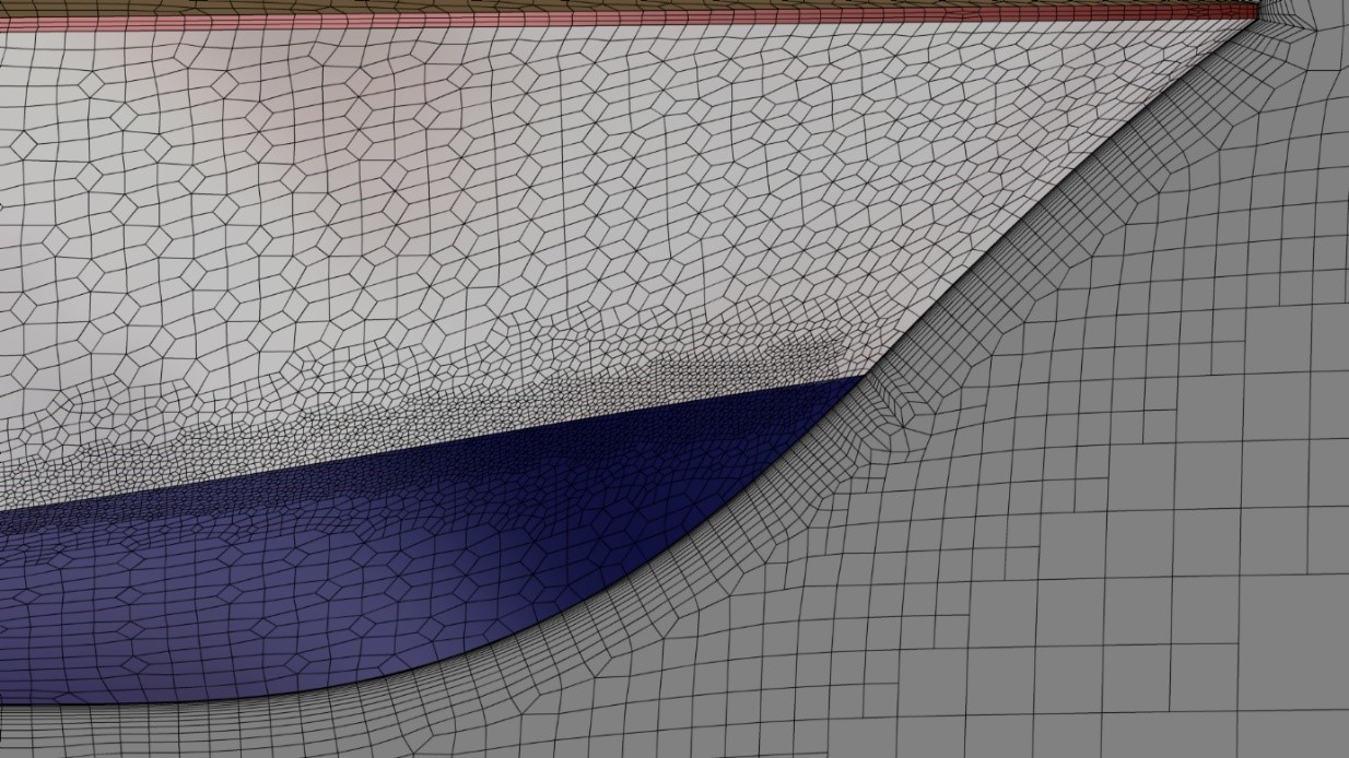 Fig.1: Close-up of the viscous layer along the hull with fixed first cell size, large number of layers and a smooth transition into the Euler mesh
 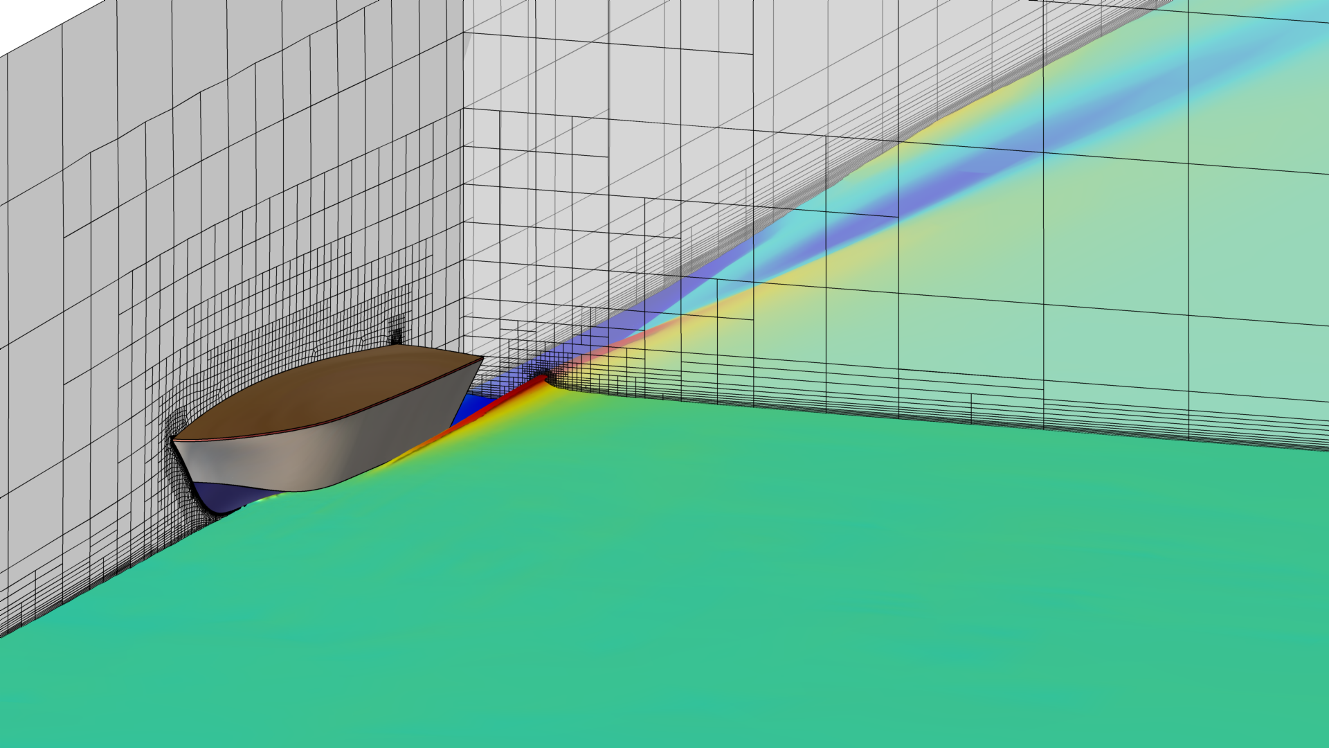 Fig.2: Free surface capturing via the adaptive grid refinement technique
 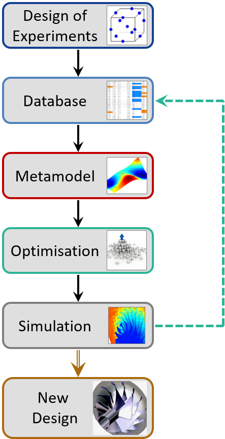 Fig.3: Optimisation strategy using a surrogate model
 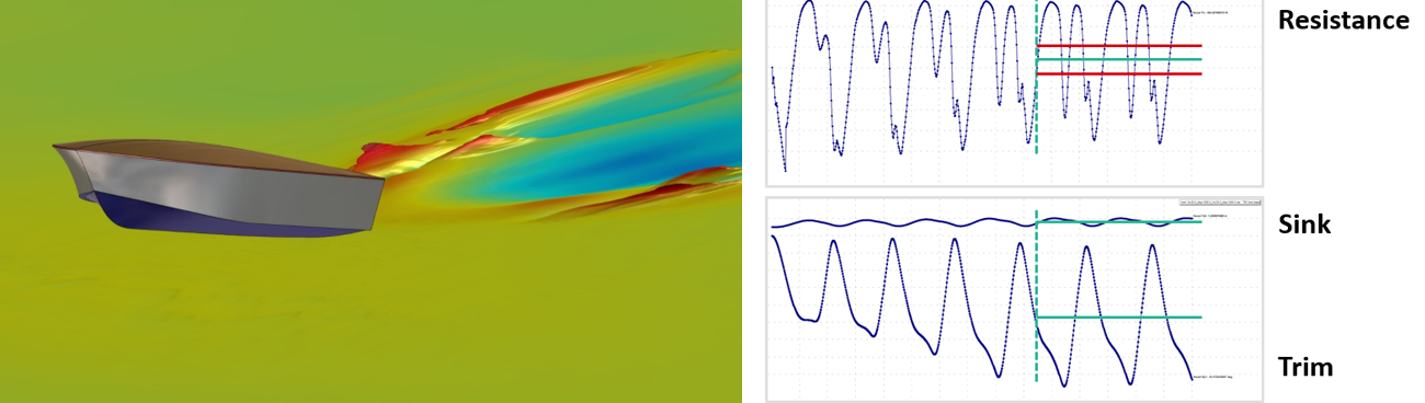 Fig.4: A sample from the database at 20m/s, flying at the last time step (and heavily slamming before)
 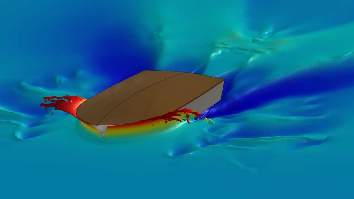 Fig.5: Worst database sample at 5m/s, producing huge bow waves and drag
 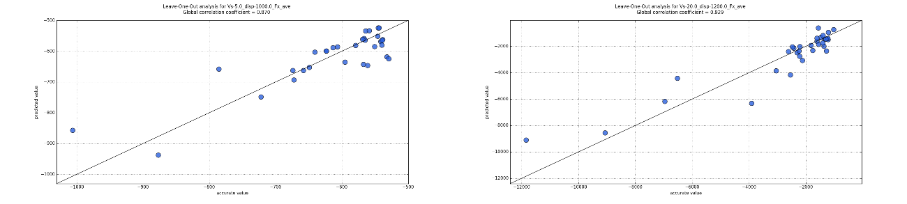 Fig.6: Leave-One-Out analysis (LOO): correlation between accurate values and approximated values from the surrogate
 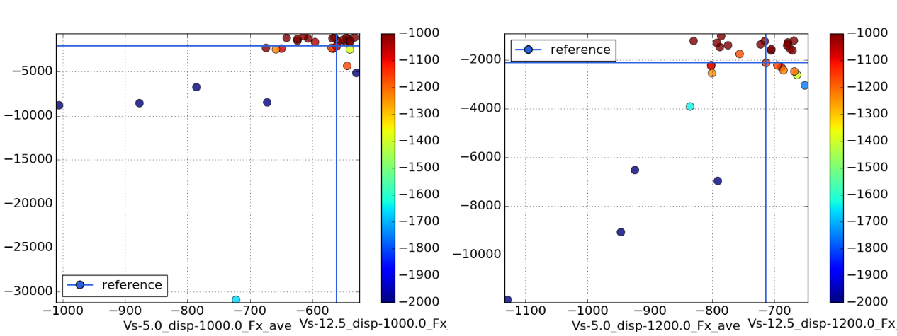 Fig.7: Total resistance of database samples (left: 1000kg; right: 1200kg). Base design is marked via the blue cross
 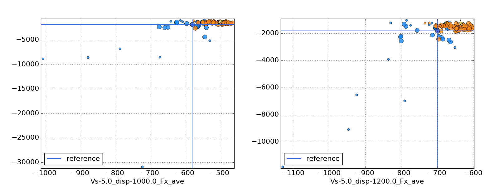 Fig.8: Total resistance of optimised samples, coloured in orange (left: 1000kg; right: 1200kg). Substantial improvements and no samples in undesired regions
 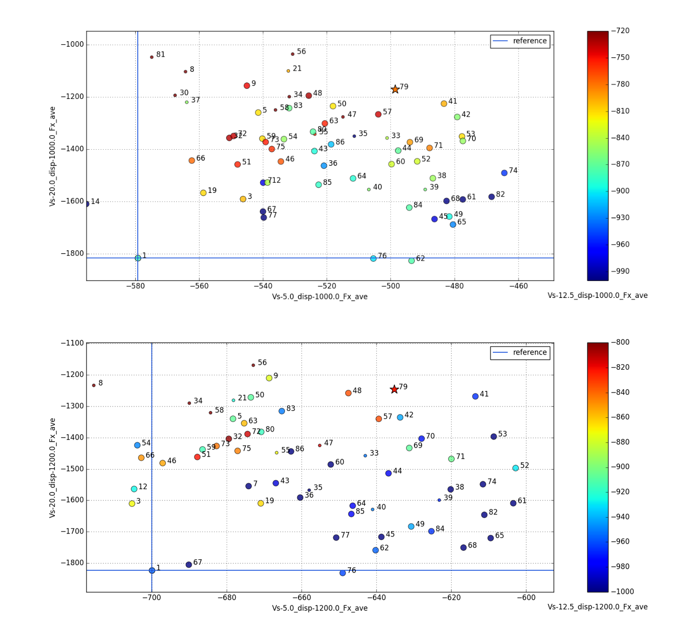 Fig.9: Total resistance values at 1000kg (top) and 1200kg (bottom). Improvements up to 35% are achieved
 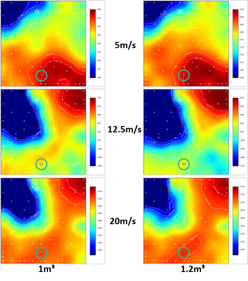 Fig.10: Self organising maps for all resistance values showing correlations and anti-correlations; the marker indicates sample #79, which is very good in all objectives
  Fig.11: ANOVA plots show dominating parameters for the total resistance values, depending on the operating conditions
  Fig.12: Hull shapes of base design and the balanced optimiser sample #79