Fully-coupled CFD Engine Simulations
Aerospace | Automotive | Turbomachinery | HVAC
The aerospace industry, like many other industries, is under pressure to drastically reduce its environmental footprint. The Flightpath 2050 goals of the European Union state that by the year 2050 all CO2 emissions per passenger kilometer must be reduced by 75%, NOx by 90% and noise pollution by 65% (relative to the year 2000). [1] One of the ways to achieve these environmental goals is by increasing turbomachinery performance. Improved analysis in the design phase, more specifically development of more reliable predictions, advancement in accuracy, inter-disciplinarity and speed of simulation tools, can add several percentage points to engine efficiency and reduce development cost and time. [2][3]
Complexity
One of the main challenges in designing an engine is the complexity in terms of geometrical details (combustion chamber features, turbine cooling holes…) and of interaction effects between the components which must be modelled with accuracy and acceptable computation time.
Full Engine Simulation Methodology
Traditionally engine design in industry has relied on tools like experimental investigation using test or flow bench set-ups, analytical models, empirical/historical data, 1D/2D codes and recently, high fidelity 3D computational fluid dynamics (CFD) for steady and unsteady flow physics modelling. Currently most of the literature work [4-6] and projects conducted at an industrial scale employ a component-by-component analysis approach, where each engine component is studied separately. Such an approach usually requires assumptions for inlet and outlet boundary conditions for each component and involves a considerable effort in coupling different component analysis tools (often with different modelling degrees of accuracy), leading to a process which is potentially error-prone from the simulation setup point of view and often resulting in significant mismatches between numerical and experimental data.
A one-way coupling approach represents one step further in increasing the accuracy of such simulations. It can be achieved, for example, by extracting outlet profiles of the flow variables from individual converged component simulations and applying them as inlet boundary condition profiles to downstream component runs. Nevertheless, the inter-component interaction is still one-way and the simulation process and results can suffer from similar drawbacks as in the totally uncoupled workflow.In the two-way coupling methodology all the components are coupled and solved simultaneously in one single simulation. This approach greatly simplifies and accelerates the simulation workflow. Since all the components are considered simultaneously, there is no need to prescribe boundary conditions between the various elements of the aero-engine. This avoids running simulations where the states at the interface between the different components have to be guessed.
The full engine CFD numerical modeling methodology can be mainly categorized in three levels:
- Steady-state RANS simulations: computationally low cost and usually involving a single meshed blade passage per turbomachinery row with mixing-plane interfaces between components
- Unsteady-state RANS time domain simulations: computationally expensive, employing several meshed blade passages per turbomachinery row, usually requiring many time steps to reach periodic flow conditions and providing solutions for a single clocking configuration per run
- Unsteady-state RANS frequency domain simulations: 2-3 orders of magnitude faster than time domain method computations, employing a single meshed blade passage per turbomachinery row, providing improved rotor-stator interfaces modeling and allowing arbitrarily clocked solution reconstruction in time.
NUMECA’s Approach to Full Engine CFD Simulation
A full 3D aerodynamic simulation of a complete gas turbine engine, applied to a micro turbine case has been conducted at NUMECA. The analysis was comprised of a single fully-coupled 3D CFD simulation for the flow of a KJ66 engine redesign. The injection and burning of fuel inside the combustion chamber are modeled with a simplified flamelet model. Using advanced RANS treatment with inputs from Nonlinear Harmonic (NLH) method (available as module for FINE™/Turbo), tangential non-uniformities are captured and the flow physics of the interaction between compressor, combustor and turbine are assessed.
Case Description
The selected test case is a redesign version of the KJ66 micro gas turbine (Figure 2). The Figure 2 shows the layout of the redesigned version of the KJ66 micro gas turbine used in the full engine computation. The centrifugal compressor is mounted at the engine entrance and it is composed of an impeller and a bladed diffuser row. The combustion chamber is followed by a high-pressure turbine (HPT), which drives the compressor, and a low pressure turbine (LPT), which would drive a propeller in an independent shaft. An exhaust hood is connected to the last LPT row at the engine exit.
Simulation Setup
The computational domain encompassed one blade passage for each turbomachinery blade row, a 60° sector for the combustion chamber (containing one fuel injector) and half exhaust hood. The three-dimensional mesh for the blade rows (compressor and turbine rows) was generated automatically using Autogrid5™, NUMECA’s turbomachinery dedicated full automatic hexahedral block-structured grid generator. The mesh for the combustion chamber and exhaust hood was generated with HEXPRESS/Hybrid™, NUMECA’s unstructured hex-dominant conformal body-fitted mesher for arbitrary complex geometries. The entire mesh has 19.20 million points.
As a first investigation, the steady RANS computation is performed with the Spalart-Allmaras turbulence model. Ambient total quantities are imposed at the engine inlet with specified axial velocity direction and static pressure is fixed at the outlet. The fuel injection is specified with static temperature and axial velocity of -120 m/s. Solid walls are assumed smooth and adiabatic. The convergence history is checked by following the evolution of the mass flow, the pressure ratio, and net torque between the HPT rotor and the impeller. The computation is launched in parallel on 144 processors on a computing cluster. In a second step, the computation is restarted with an improved rotor-stator connection based on the NLH method.
Combustion Model
The injection and burning of fuel inside the combustion chamber are modeled with a simplified flamelet model implemented in OpenLabs™. With this model, an additional equation is solved for the mixture fraction f, with the flame temperature as function of the composition.
Results
Steady-state Computation
The convergence history of mass flow rate error between the engine inlet and outlet drops to less than 0.2% after 25000 iterations in approximately 24 hours of wall clock time. The net torque Mz reaches a final value of +0.21 N.m when the couple impeller-HPT rotor spins at -80000 rpm, meaning that the turbine produces enough torque to drive the compressor and both components are very close to be load balanced.
Figure 4 shows the static pressure, static temperature and absolute Mach number distributions at midspan of the compressor and turbine as well as in the solid walls of the combustion chamber and exhaust hood. The flow fields are continuous across the machine with a gradual raise of Mach number through the impeller and subsequent conversion of the kinetic energy into pressure across the diffuser. At approximately 160 kPa, air reaches the combustion chamber where the simulated combustion process takes place with a relatively small pressure loss. The maximum temperature at the combustion chamber is around 2200K at the combustor inner chamber. The hot gases from the combustion enter the HPT at approximately 983K and are expanded through the downstream blade rows, exiting the machine at 932K.
As shown in the Figures 5, the mixture fraction color contour successfully depicts the fuel stream entering the combustion chamber with f = and the combustion gases gradually reaching a value of 0.02 at the component exit. The effect of the holes in the inner chamber walls can be noticed in the magnitude of velocity color contour: they provide a flow of compressed air, acting as oxidizer for the combustion process, to mix with vaporized fuel and achieve ignition.
NLH Computation
The results from the RANS computation using a mixing plane treatment at the rotor stator interface can be compared to the results of the NLH analysis. In particular, it is interesting to note the effect of the improved connection approach with respect to the inter-components interactions.
Figures 6 and 7 show similar results on the mass flux for both simulations at the exit of the combustion chamber. A pattern linked to the periodicity of the fuel pipes and to the combustion zones can be observed. The transfer of information from the combustor outlet to the adjacent downstream HPT nozzle is different for the RANS simulation and its NLH counterpart. The mixing plane approach shows no tangential non-uniformities, while the NLH rotor-stator treatment proves to be a low cost first step in capturing tangential non-uniformities.
The Figure 8 shows the results for absolute total enthalpy and mixture fraction at the HPT and LPT inlet connections. The azimuthal averaging used in the mixing plane approach, where tangential non-uniformities are not perceived by downstream components, can be noticed for the RANS simulation. In contrast, the Fourier decomposition together with the local non-reflective boundary treatment used in the NLH method is able to show a slight improvement at the interfaces.
Conclusions
A successful simulation of the three-dimensional flow of a complete micro gas turbine engine has been achieved, on the basis of a fully-coupled 3D CFD simulation of a redesigned version of the KJ66 micro gas turbine. Compared to the component-by-component analysis, the fully coupled approach enables the solution of the whole engine in one single simulation. Furthermore it simplifies the simulation workflow as only the engine inlet and outlet pressures, the rotating speed and the fuel mass flow rate need to be prescribed.
Source: Mateus Teixeira, Luigi Romagnosi, Mohamed Mezine, Yannick Baux, Jan Anker, Kilian Claramunt, Charles Hirsch A Methodology for Fully-Coupled CFD Engine Simulations, Applied to a Micro Gas Turbine Engine. ASME. Turbo Expo: Power for Land, Sea and Air, Volume 2C: Turbomachinery ():V02CT42A047. doi:10.1115/GT2018-76870.
References
[1] Flightpath 2050: Europe’s Vision for Aviation, 2011, http://www.acare4europe.org/sria/flightpath-2050-goals.
[2] National Academies of Sciences, Engineering, and Medicine, 2016, “Commercial Aircraft Propulsion and Energy Systems Research: Reducing Global Carbon Emissions”, Washington, DC: The National Academies Press
[3] Mavriplis D., Darmofal D., Keyes D., Turner M., 2007, “Petaflops opportunities for the NASA Fundamental Aeronautics Program”, 18th AIAA Computational Fluid Dynamics Conf., Miami, FL, AIAA paper 2007–4084.
[4] Xiang J., Schluter J. U., Duan F., 2016, “Study of KJ-66 Micro Gas Turbine Compressor: Steady and Unsteady Reynolds-Averaged Navier–Stokes Approach”, Proceedings of the Institution of Mechanical Engineers Part G Journal of Aerospace Engineering.
[5] Gonzalez C.A., Wong K.C., Armfield S., 2008, “Computational study of a micro-turbine engine combustor using large eddy simulation and Reynolds averaged turbulence models”, ANZIAM J. 49 (EMAC2007) pp.C407–C422, C407.
[6] Turner M., 2000, “Full 3D Analysis of the GE90 Turbofan Primary Flowpath”, NASA/CR—2000-209951.
Products
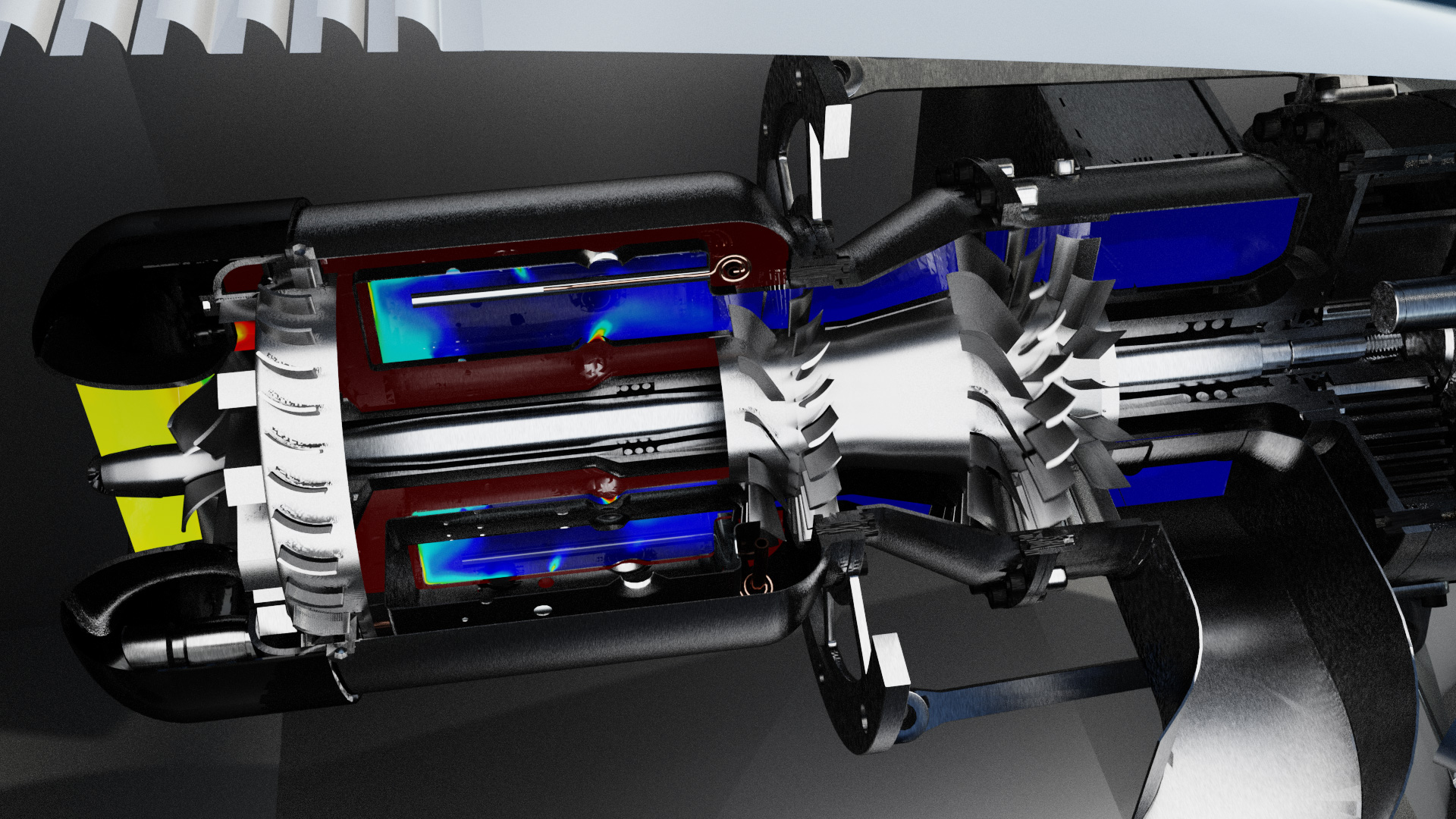
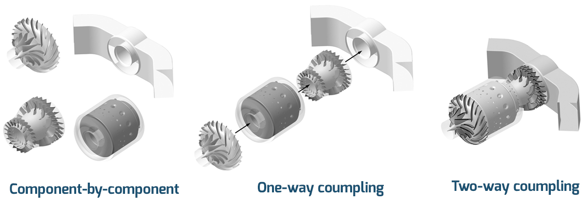 FIGURE 1: Three types of full engine simulation methodologies
  FIGURE 2: Layout of the KJ66 micro gas turbine
 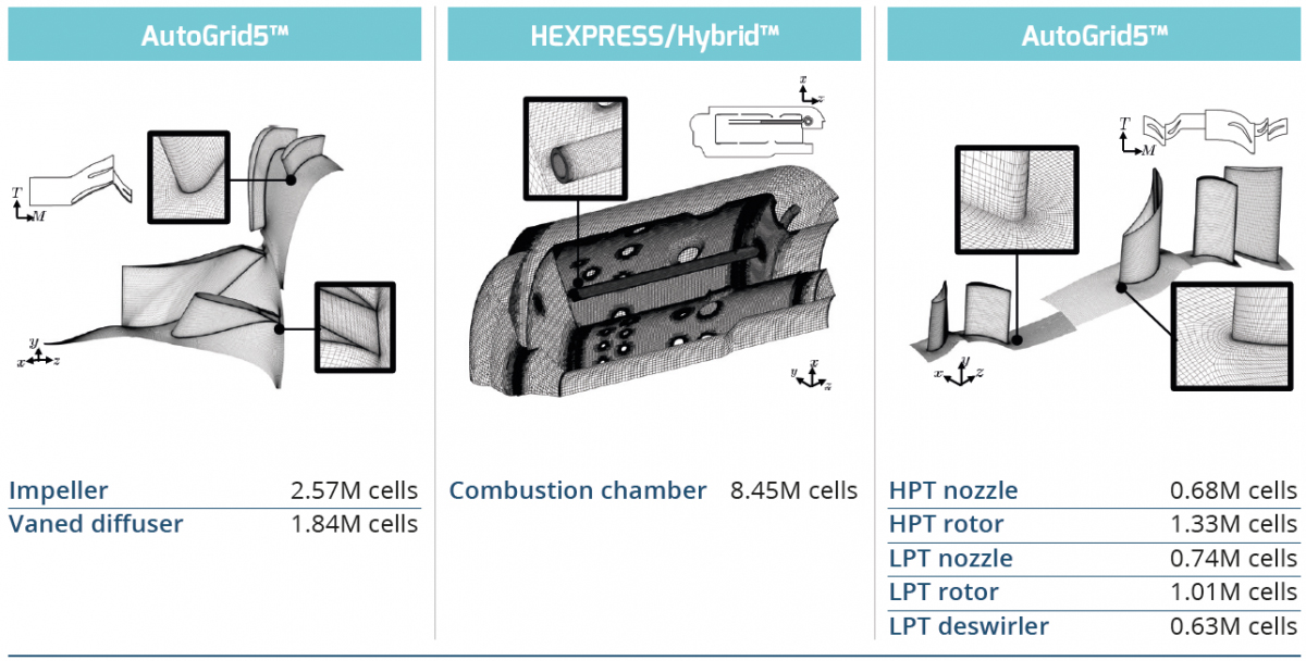 FIGURE 3: Compressor, combustion chamber and turbine 3D mesh view and blade-to-blade layout (shrouds are omitted).
 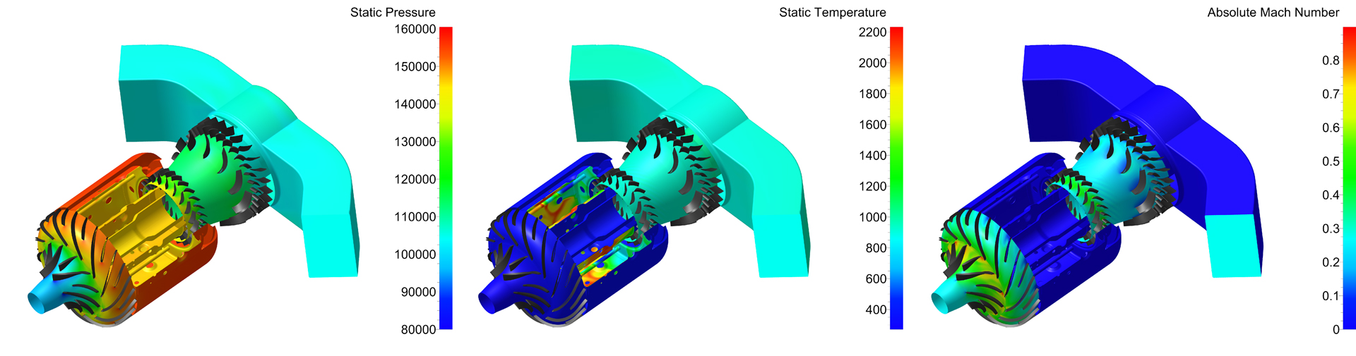 FIGURE 4: Static pressure, static temperature and absolute Mach number distributions at midspan of the compressor and turbine as well as in the solid walls of the combustion chamber and exhaust hood.
 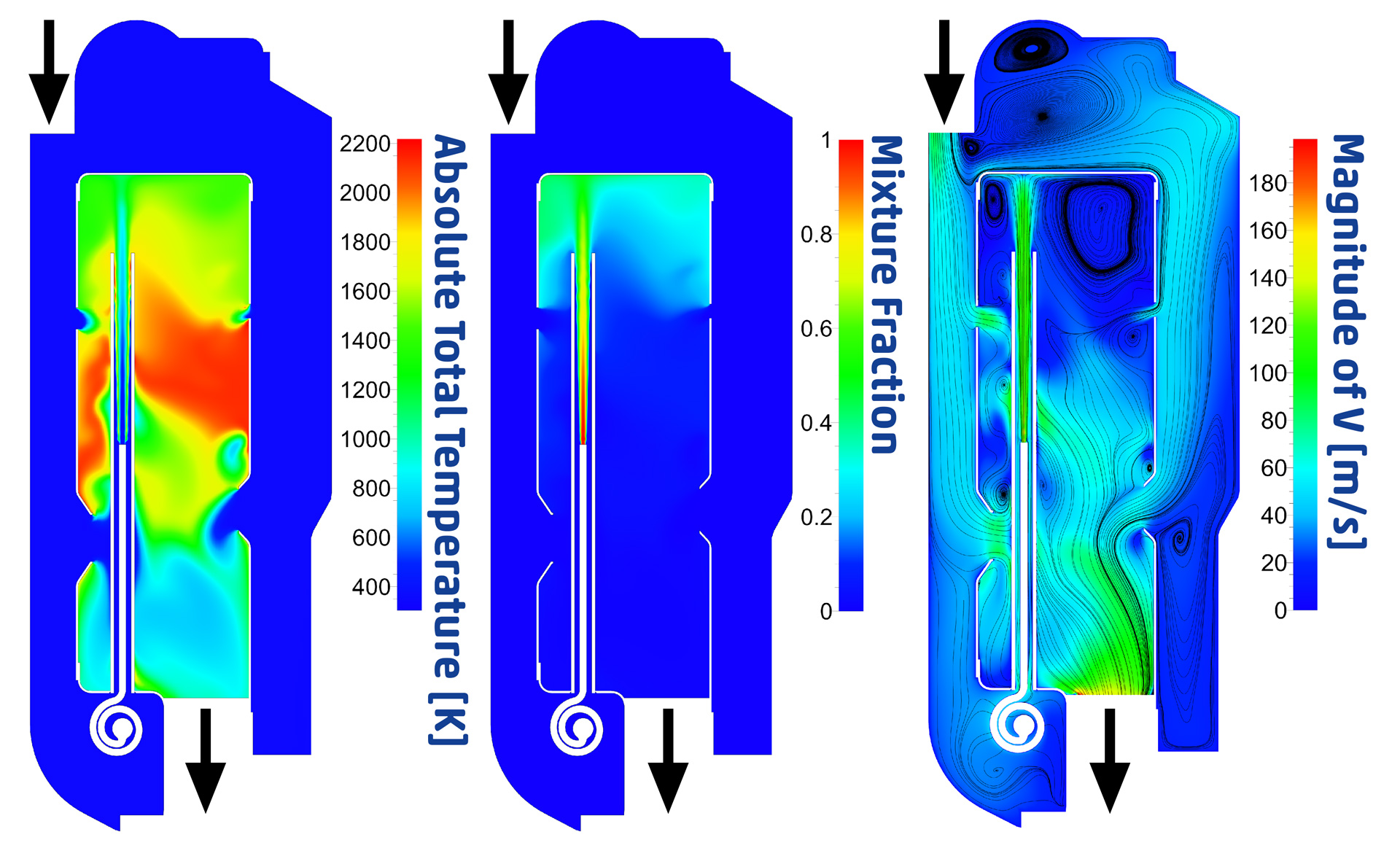 FIGURE 5: Absolute total temperature, mixture fraction and magnitude of absolute velocity distribution at the meridional plane of the combustion chamber.
 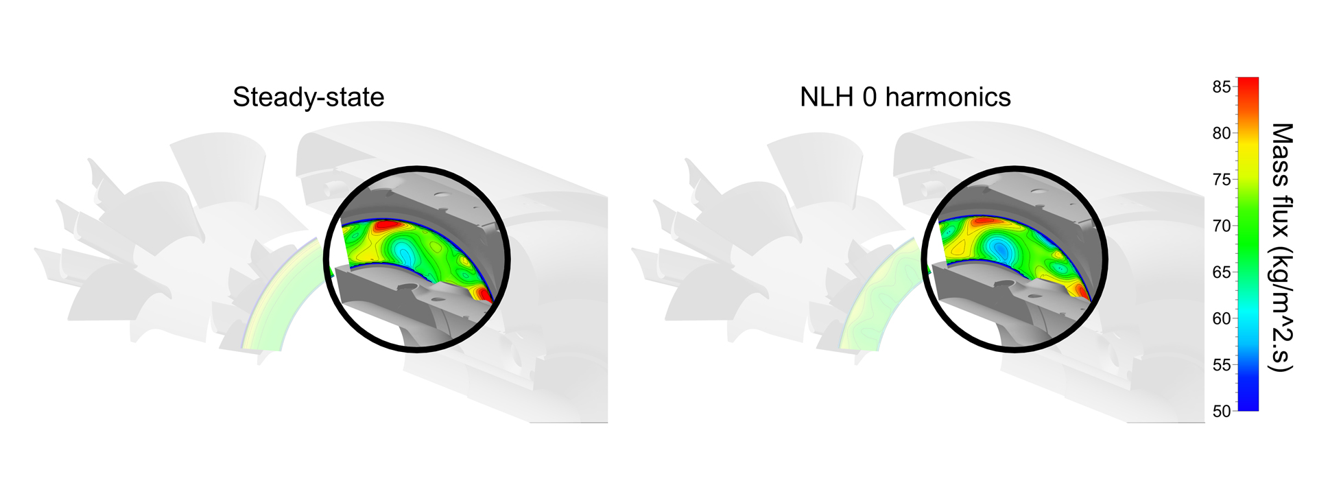 FIGURE 6: Mass flux at the outlet of the combustion chamber and at the inlet of the HPT for the steady-state (left) and NLH 0 harmonic (right) simulations.
 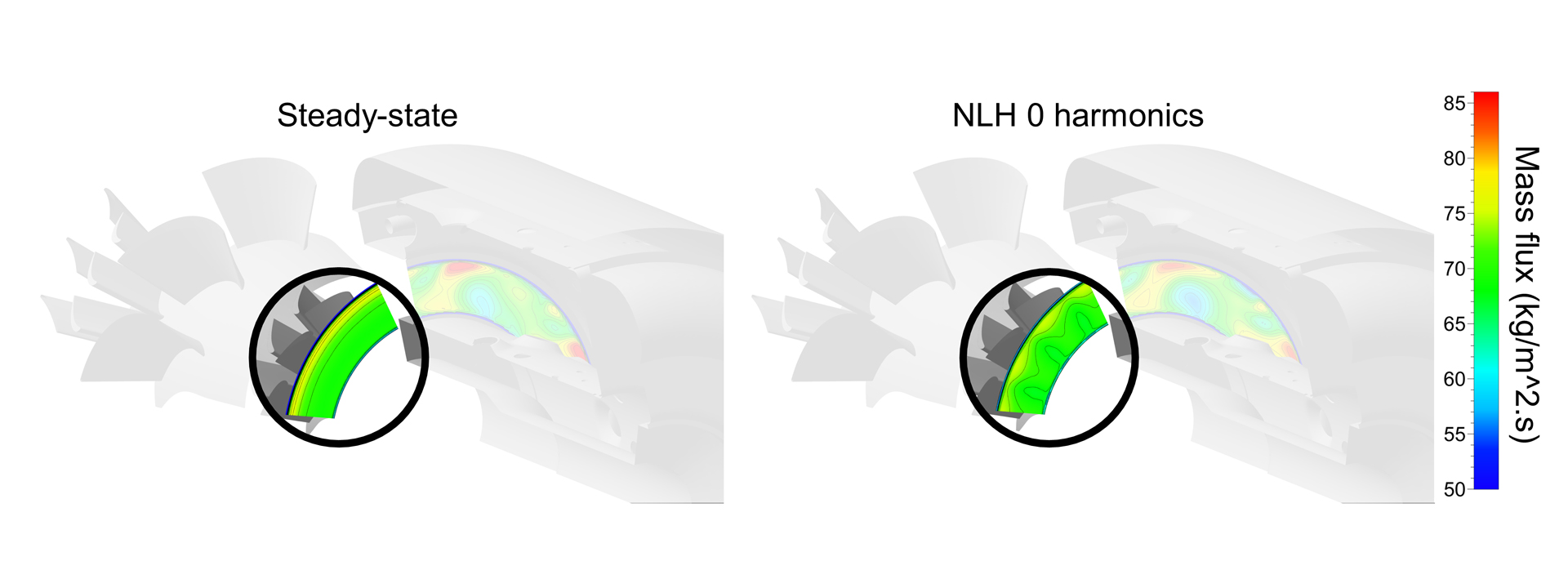 FIGURE 7: Mass flux at the outlet of the combustion chamber and at the inlet of the HPT for the steady-state (left) and NLH 0 harmonic (right) simulations.
 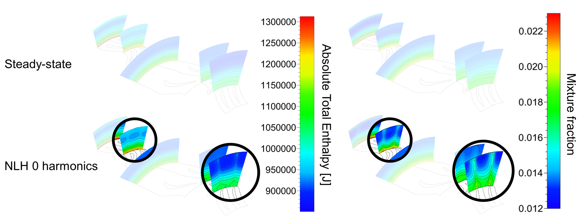 FIGURE 8: Absolute total enthalpy and mixture fraction at the inlet of the HPT and LPT blade rows for the steady-state (top) and NLH 0 harmonic (bottom) simulations.